Project Summary

For this project, we want a bot to play the Snake game and achieve reasonably high score.

Without ML, we can use rule-based approach using a hard-coded fixed set of rules. For example, we can use an algorithm that will pick the shortest path to food. However, as the snake grows, said algorithm will not be able to avoid biting itself. Of course, we can program a new set of rules to tackle this specific scenario, but even so, this shows that rule-based approach lack adaptability and scalability. For a game with large state space like Snake, we cannot satisfy all possible scenarios.

Reinforcement learning (RL) overcomes these limitations by learning effective strategies directly from experience, without requiring explicit programming of game-specific heuristics. Unfortunately, RL is not a silver bullet to this problem. In fact, our RL implementation did not yield satisfying result. Nevertheless, taking all of the above factors into consideration, we believe that RL is the right step toward a better solution to solving Snake game.

Approach

1. General Overview

For this project, we employ Reinforcement Learning (RL) to train an AI agent to play the Snake game effectively. Given the large state-space of the game (numerous possible configurations of the snake and fruit on the grid), we opt for policy-based, model-free RL methods. Specifically, we consider two algorithms: Advantage Actor-Critic (A2C) and Proximal Policy Optimization (PPO), both implemented via the Stable-Baselines3 library. These algorithms directly learn a policy (a mapping from states to actions) without modeling the environment’s dynamics, making them suitable for our scenario.

• Environment: We set up a Gymnasium environment to simulate the Snake game, defining the observation space, action space, and rewards, and then training the A2C and PPO models to maximize the snake’s score.
• Training:
  • In phase 1, we train and compare the performance of A2C and PPO in order to choose one to go forward. The reason for this is due to our limitations in time and resources.
  • In phase 2, we use the chosen algorithm to train models for various scenarios and evaluate their performance.

2. Setting Up the Snake Game Environment

We use Gymnasium to create a custom RL environment for the Snake game. The environment is defined as follows:

• Observation Space: A 3D NumPy array of integers representing the game arena. Each cell in the grid is assigned a value:
  • 0 for empty space
  • 1 for the fruit
  • 2 for the snake’s body
  • 3 for an obstacle block
  • 4 for the extra fruit The array’s dimensions are [height, width, channels], where channels encode the state of each cell.
• Action Space: Discrete with four possible actions: {0: Up, 1: Down, 2: Right, 3: Left}.
• Terminal State: The episode ends if the snake hits the wall (goes outside the arena), or collides with its own body, or collides with an obstacle block.
• Reward Function:
  • +1 when the snake eats the fruit (increasing its length and score). If there is an extra fruit, then the reward for the main fruit will be +0.2, and for the extra fruit will be +0.8
  • -1 when the snake reaches a terminal state
  • 0 otherwise (for each step where no fruit is eaten and the game continues)

The Gymnasium environment includes the following key methods:

• step(action): Updates the environment based on the given action. The snake moves in the specified direction (Up, Down, Right, or Left). If the action is invalid (e.g., reversing direction into itself), the snake continues in its current direction. Returns the new observation, reward, and whether the episode has ended.
• reset(): Resets the environment to an initial state. The score is set to zero, the snake starts with a length of 1, and its position and the fruit’s position are randomly initialized within the arena.
• render(): Generates an RGB image of the current arena for visualization.
• close(): Terminates the environment.

This setup provides a clean interface for the RL algorithms to interact with the game.

3. Training Process

3.1. PHASE 1

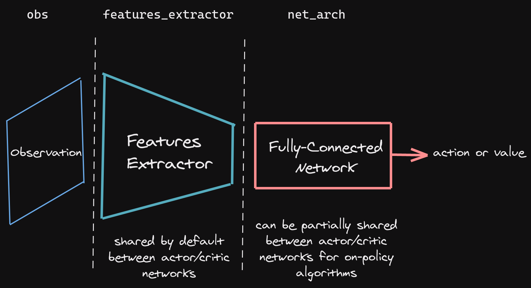
We train two separate models using A2C and PPO from Stable-Baselines3 to compare their performance. Both algorithms process the observation space (the 3D grid) as an image input, using a convolutional neural network (CNN) as a feature extractor to convert the raw grid into a feature vector representing the current state s. This vector is then fed into a policy network to select an action a. The policy network architecture follows the default CNN setup in Stable-Baselines3, as shown below:

Below, we explain how A2C and PPO work and how we apply them to the Snake game.

3.1.1. Training with A2C

A2C is an actor-critic method that combines policy-based and value-based RL. It uses two networks:

• Actor: Learns the policy π(a|s; θ)—the probability distribution over actions given a state. It selects actions to maximize expected rewards.
• Critic: Estimates the value function V(s; w), which predicts the expected cumulative reward from a given state.

The algorithm updates the actor using the advantage function, defined as: [ A(s, a) = Q(s, a) - V(s) ] where ( Q(s, a) ) is the action-value function (approximated via the reward received and bootstrapped future rewards), and ( V(s) ) is the state-value function from the critic. The advantage measures how much better an action is compared to the average action in that state.

The actor’s policy is updated by maximizing the objective: [ J(θ) = E[log π(a|s; θ) * A(s, a)] ] using gradient ascent. Meanwhile, the critic minimizes the loss: [ L(w) = E[(r + γ * V(s’) - V(s))^2] ] where r is the reward, γ is the discount factor (set to 0.99 by default), and s' is the next state.

For the Snake game, A2C takes the 3D observation grid, extracts features with the CNN, and outputs action probabilities (e.g., 25% Up, 25% Down, etc.). We train for 10 million timesteps, using Stable-Baselines3’s default hyperparameters: learning rate = 0.0007, n_steps = 5 (steps per update), and and our gamma = 0.9. These values are sourced from the library’s documentation, and we did not tune them further due to computational constraints.

3.1.2. Training with PPO

PPO is a more stable policy gradient method that improves on A2C by constraining policy updates to avoid large, destabilizing changes. Like A2C, it uses an actor-critic framework but introduces a clipped objective function to limit how much the policy can change in each update.

The PPO objective is: [ J(θ) = E[min(r(θ) * A(s, a), clip(r(θ), 1-ε, 1+ε) * A(s, a))] ] where:

• ( r(θ) = π(a

  s; θ) / π_old(a

  s; θ_old) ) is the probability ratio between the new and old policies,

• ( ε ) is the clipping parameter (default = 0.2),
• ( A(s, a) ) is the advantage, calculated similarly to A2C.

The clipping ensures that the policy doesn’t deviate too far from the previous version, improving training stability. The critic’s loss is the same as in A2C.

For the Snake game, PPO processes the observation grid similarly to A2C, using the same CNN feature extractor. We train for 10 million timesteps with default hyperparameters from Stable-Baselines3: n_steps = 2048, clip_range = 0.2, and our gamma = 0.9 and learning rate = 0.00025. These defaults are well-documented and widely used, so we kept them unchanged.

3.1.3. Comparison and Limitation

• As shown in the graph below, A2C performs better than PPO within the first 10 mil steps, in the default arena. Hence, we opt to only perform evaluation on models trained by A2C.

  

3.2. PHASE 2

Using the same A2C algorithm, we train different models for different scenarios to see how they perform. However, we use our custom CNN architecture instead of the default one by SB3. We also made a few adjustment to our training environment due to technical limitations. Details regarding these adjustments can be found in the “Hyper-parameters and Reproducibility” section down below.

Here are the scenarios that we trained our models in:

1. Arena default: empty 8x8 arena.
2. Arena with an extra fruit:
   • Every time a normal fruit spawn, there is a 50% chance of spawning an extra fruit.
   • If there is no extra fruit spawned, then the reward for the normal fruit will be +1.
   • If there is extra fruit spawned, then the reward for the normal fruit will be +0.2, and the reward for the extra fruit will be +0.8.
   • If the normal fruit is eaten before the extra fruit, the extra fruit will disappear.
3. Arena with a rectangle obstacle in the middle.
   • For this scenario, we found out that removing the penalty for terminal state will help the model learn better.
   • As such, we trained our model using the default setup with no penalty for terminal state.
4. Arena split by half by a wall with a hole in the middle.
   • For this scenario, we found out that removing the penalty for terminal state will help the model learn better.
   • As such, we trained our model using the default setup with no penalty for terminal state.

3.2.1. Custom CNN Architecture

For Phase 2, we developed a custom CNN architecture inspired by both ResNet and the Llama model architecture, incorporating modern deep learning techniques to improve performance. Our custom architecture features several key components:

1. SwiGLU Activation Function: Instead of traditional ReLU activations, we implemented SwiGLU (Swish-Gated Linear Unit) as described in the “GLU Variants Improve Transformer” paper. SwiGLU combines the benefits of gating mechanisms with smooth activation functions, allowing for better gradient flow during training.

2. Residual Connections: Following ResNet’s design philosophy, we incorporated residual connections that enable the network to learn identity mappings more easily, helping to address the vanishing gradient problem in deeper networks. These connections allow information to flow directly from earlier layers to later ones, facilitating both faster training and better performance.

3. Enhanced Feature Extraction:

   • A larger initial convolutional layer with a 7×7 kernel to capture more spatial information
   • Multiple residual blocks to maintain and refine feature representations
   • Strategic max pooling to reduce spatial dimensions while preserving important features
   • A final SwiGLU-activated linear layer to produce the feature vector

The architecture processes the game state (represented as a grid) through these components to extract meaningful patterns that inform the agent’s policy and value functions.

In our experiments, this custom architecture demonstrated significantly faster learning compared to the default SB3 implementation used in Phase 1. The model achieved approximately 7 points on average in just 2.5 million training steps, compared to approximately 5 points after 10 million steps with the original architecture.

This dramatic improvement in early training efficiency suggests that the residual connections help the network learn basic game patterns more quickly, while the SwiGLU activations may provide better gradient flow that facilitates more effective policy updates. While the final performance after extended training may converge to similar levels, the custom architecture’s ability to reach good performance with 75% fewer training steps represents a substantial improvement in computational efficiency.

4. Hyper-parameters and Reproducibility

4.1. PHASE 1

The models are trained using A2C and PPO, and the default CNN architecture from Stable-Baselines3 (two convolutional layers followed by a fully connected layer). Our hyper-parameters for A2C and PPO models are:

• n_steps = 2048
• clip_range = 0.2
• gamma = 0.9
• learning_rate = 0.00025

We train each model for 10 million timesteps, which corresponds to roughly 10 million interactions with the environment (though episodes terminate earlier upon failure). The training data is generated on-the-fly by the Gymnasium environment, so no external dataset is required. For reproducibility, we set a random seed of 42 in both the environment and the algorithms.

4.2. PHASE 2

Similar to phase 1, except:

• We use our custom CNN architecture (three convolutional layers followed by a fully connected layer) instead of the default one by SB3.
• We adjust our arena size from 10x10 to 8x8 for faster train-and-test iterations.

Evaluation

1. PHASE 1

We plan to evaluate performance by comparing the average score (total fruit eaten per episode) across 100 test episodes for each model after training.

1.1. A2C model

• Training evaluation: As shown in fig 02, we observed a mean fluctuation of around 1. Interestingly, we noticed a significant jump in mean score between 3 mil and 4 mil steps. At the end of training, we observed a mean score of 4.18.

• Final evaluation: During final evaluation, we observed a mean reward of approximately 7.

  

1.2. PPO model

• Training evaluation: As shown in Fig 02, we observed a mean fluctuation of around .3. Noticably, there is a jumped in mean score at the beginning. At the end of training, we observed a mean score of 4.7.

• Final evaluation: During final evaluation, we observed a mean reward of approximately 4.8

  

1.3. Observation

• Looking at Figure 2, A2C model performs better than PPO model throughout the training process, as well as final evaluation.

  

• A problem with A2C model is that at first, it wastes lots of the time for little returns. Figure 5 show the mean episode length for A2C model is much higher and fluctuating than PPO model in the beginning. Yet during those same timesteps, PPO model gets better mean rewards.

2. PHASE 2

We plan to evaluate performance of our models using the average score (total fruit eaten per episode) across 400 test episodes, as well as the statistics during the training process.

2.1. Arena default:

• During training, our new A2C model in phase 2 achieves better average reward than the A2C model in phase 1 (~7 pts vs. ~5 pts), and much faster (2.5 mil steps vs. 10 mil steps).

  

• In the final test, the new A2C model achieves ~7.3 points on average.

  

2.2. Arena with rectangle obstacle:

• For this scenario, if we enable penalty for terminal state, the model will not learn at all. Therefore, we opt to turn off the penalty.
• We use two sizes of the obstacle: 4x4 and 2x2.

  Obstacle 4x4:

  • During training, the model initially has a trajectory similar to the default scenario. However, the result plummets half-way through. At the end of training, the model achieves ~3.5 points on average.

    

  • In the final test, the model achieves ~3 points on average.

    

  Obstacle 2x2:

  • During training, the model initially performs worse than the default scenario. However, the model then improves and surpass the performance of the default scenario. At the end of training, the model achieves ~9 points on average.

  • A possible explanation to this surprising behavior is that, the obstacle actually guides the model to learn to move in a spiraling pattern - which has a better chance of surviving than randomly turning and bite itself by accident.

2.3. Arena split by half by a wall with a hole:

• For this scenario, we opt to turn off the penalty. We choose a hole 1/4th the size of the wall.

• During training, the model performs arguably well and similar to the scenario without wall. At the end of of training, the model achieves ~5.2 points on average.

  

• In the final test, the model achieves ~4.9 points on average.

  

• If we enable penalty for terminal state, the model will never cross the wall, as the penalty will discourage the snake from exploring the hole.
• In that case, if a fruit appear on the snake’s side, the snake will grab the fruit. Otherwise, it will spin at the same spot until times out.

2.4. Arena with extra fruit:

• The extra fruit worth 0.8 point while the normal fruit worth 0.2 point. If the model only eats normal fruit first, the extra fruit will disappear, the model will lose out points, and the average score will tank heavily.

• However, during training, while the model had a slower start at first, its average reward eventually improves. At the end of training, the model in “extra fruit” scenario performs noticeably similar to the model without extra fruit.

  

• We can also observe the behavior when pairing this scenario with another scenario. For example, for the scenario with obstacle, we can also add extra fruit. The performance with and without extra fruit are pretty similar.

  

• In the final test for default arena with extra fruit, the model achieves ~5.7 points on average.

  

• As such, we can see that the model consistently learns to prioritize the extra fruit over the normal fruit.

Resources Used:

• Snake Game by PavanAnanthSharma
• Gymnasium for RL environment and documentation.
• Stable-Baseline3 for A2C and PPO implementation, and documentation.
• Series on RL Basics by Luke Ditria
• Blog on PPO Implementation details
• Tensorboard for data visualization.

AI Tool Usage:

• We used ChatGPT to improve the “Summary” section of this report.